


반응형
Learing for classification => class를 나누는 경계선을 찾는 문제였음
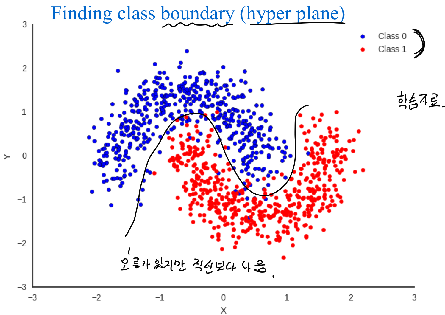
경계선을 직선으로 할 경우 오류가 많지만 곡선으로 할 경우 오류가 줄어들음
Scikit-learn classifiers
- Logistic regression
- KNN'
- Support Vector Machine (SVM)
- Naive Bayes
- Decision Tree
- Random Forest
- AdaBoost
- xgboost(Not in scikit-learn)
여러 classifier들이 있지만, 어떤 방법이 현재 가지고 있는 데이터에 대해 가장 효과적인지 사전에 알 수 없다. 따라서 모든 방법을 해보고 그 중에 좋은 것을 선택해야한다.
1. Decision Tree
- 큰 문제를 작은 문제들의 조각으로 나누어 해결한다.
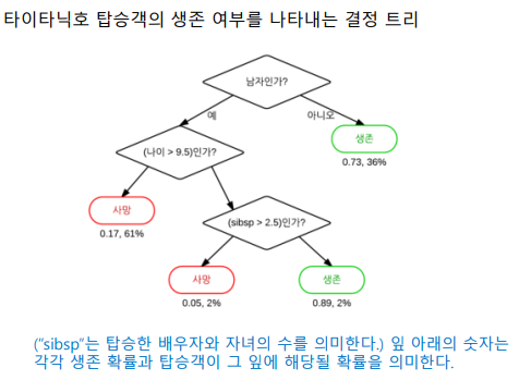
- 예측을 위한 모델이 만들어졌을때, Tree의 형태로 나온다.
- Tree형태이기때문에 결론이 나온 이유를 이해하기 쉽다. => 예측 결과에 대해서 근거가 명확하다
- 예를 들면 의료분야에서 질병진단시 근거가 명확해야한다.
1.1 Decision Tree 예시
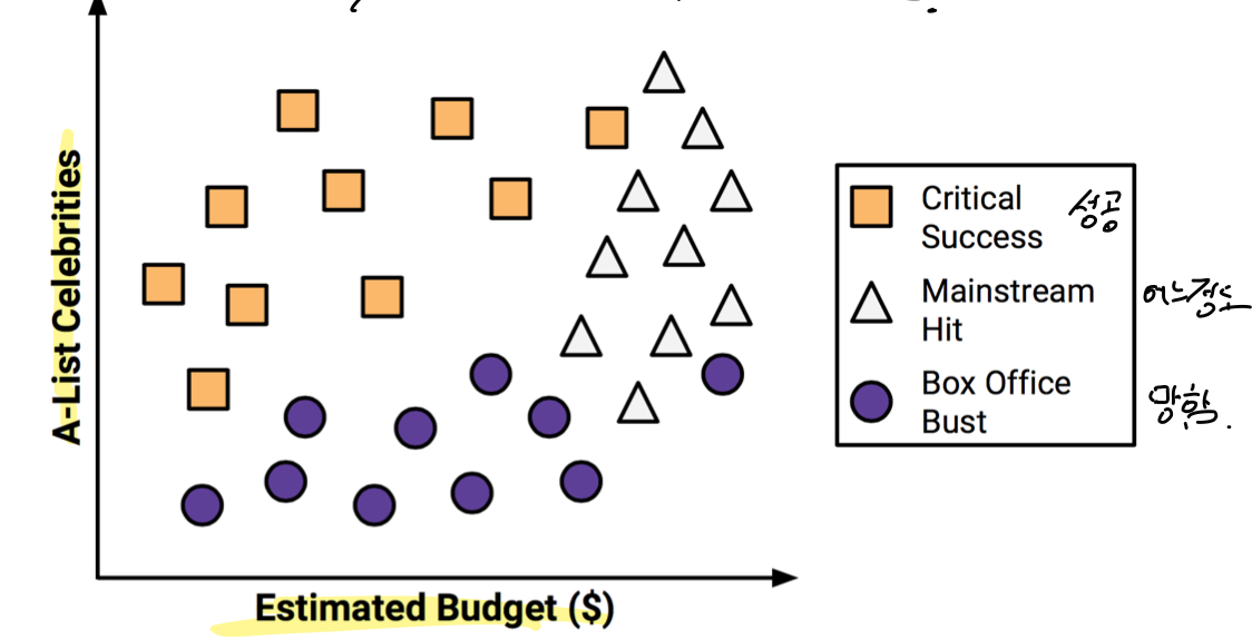
- 영화 대본 및 기본 정보를 이용하여 영화가 흥행할지 예측하는 모델
- 유명 배우수와 추정 제작비로 예측
- 결과는 매우흥행, 어느정도 흥행, 폭망으로 3가지로 구분
- 특정 class와 다른 class를 가장 잘 구분할 수 있는 선을 찾는다. 하지만, 잘못 예측한 경우도 있다.
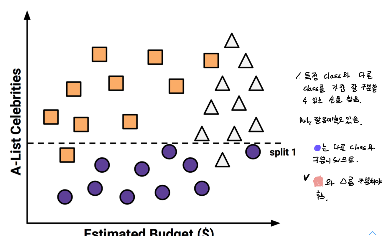
- 다른 class를 다시 구분하는 선을 찾는다. 잘못 예측한 것들이 있지만 최선이다.
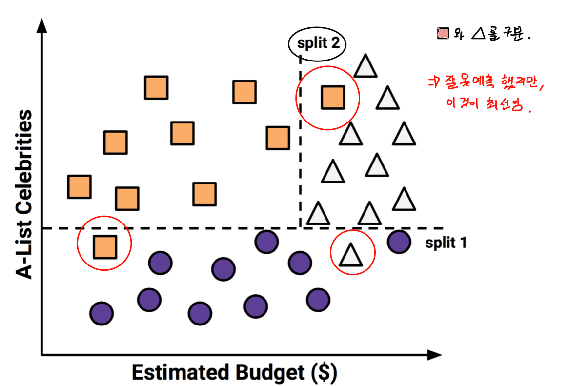
- 결과

1.1.1 문제점
- 트리의 node를 선택 할 때 데이터 셋에서 어떤 속성을 선택할 것인가?
=> 이전 영화문제에서는 유명배우가 많으면서 예산이 적어야 성공한 영화였다. 그러면 스타급 배우수가 먼저인가? 예산이 먼저인가?
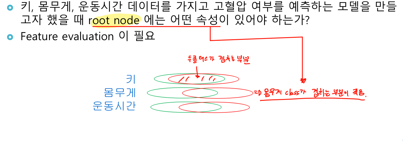
사진과 같이 class가 겹치는 부분이 적은 것을 선택한다.
- 트리를 split할 때 언제 중단할 것인가?
=> 트리의 가지를 계속 뻗어나가면 모든 instance를 100%t식별 할 수 있다. 하지만 overfitting발생
적당할 때 트리생성을 중단 해야한다. -> 가지치기(pruning)
경계선을 많이 나누면 이론상으로 100% 예측 가능한 tree를 만들 수 있다. 하지만 test 정확도는 낮다.
1.1.2 장점
- 모든 문제에 적합
- 결측치, 명목속성(범주), 수치속성을 처리하기에 용이
- 여러 속성중 중요한 속성들만 사용하여 예측
- 매우 많은 수 또는 상대적은 훈련 데이터로도 모델 구축 가능
- 수학적 배경이 없이도 해석이 가능한 모델
- 단순한 이론적 근거에 비해 높은 효율성
1.1.3 단점
- 결정 트리는 다수의 레이블을 가진 속성쪽으로 구분하는 경향이 잇음
- 모델이 쉽게 과적합(overfitting)하거나 과소적합(underfitting) 됨
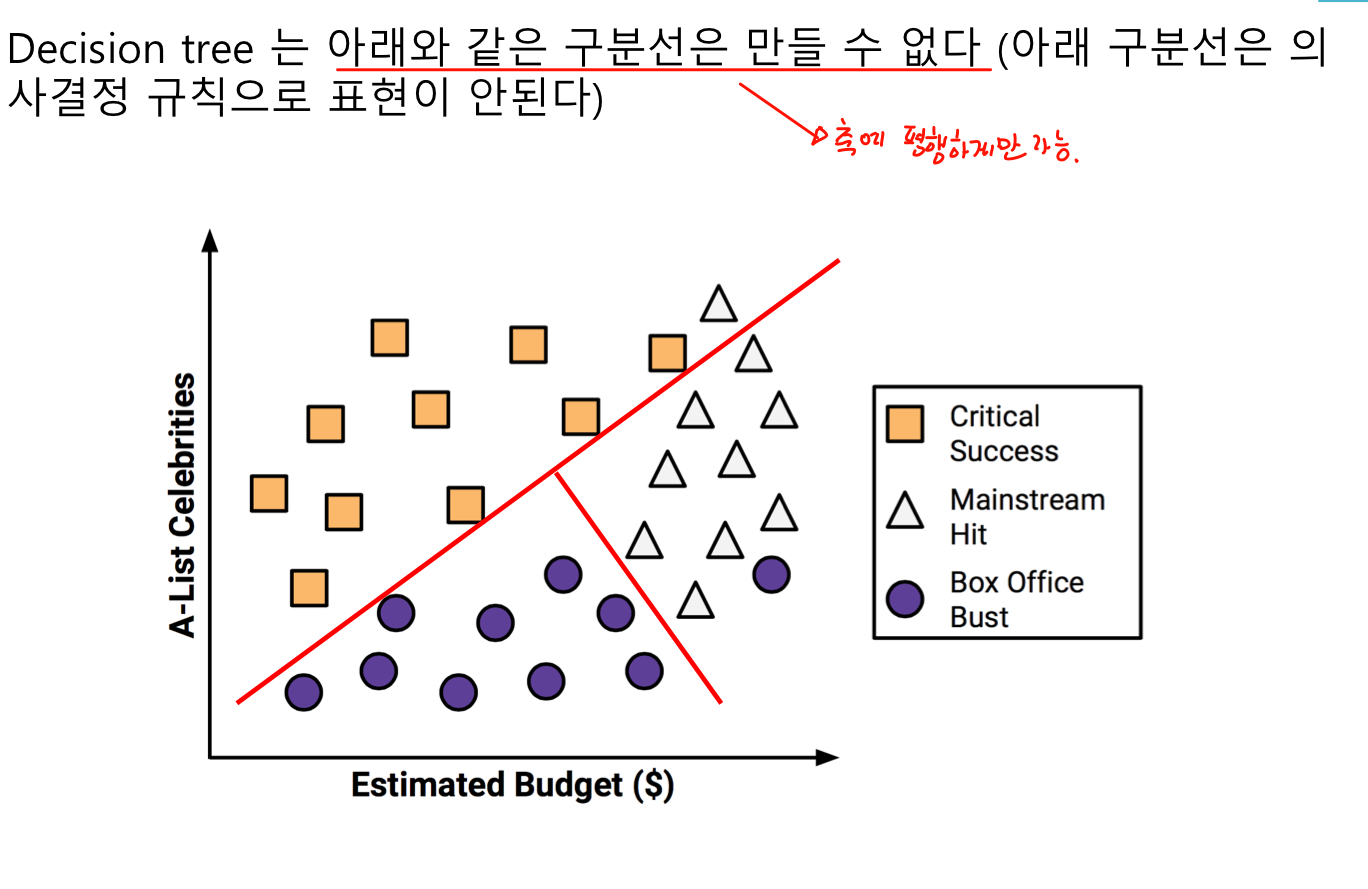
- 축에 평행한 구분선을 사용하기 때문에 일부 관계를 모델화 하는데 문제가 있다.
- 훈련 데이터에 대해 약간의 변경이 결정 논리에 큰 변화를 준다.
- 큰 트리는 이해하기 어렵고 직관적이지 않다.
1.1.4 코드
예시) liver.scv (간 장애 자료, 레이블 + 혈액검사 결과(6개 변수))
category
mcv
alkphos
sgpt
sgot
gammagt
drinks
category = 클래스 정보. 0 : 정상 1 : 간장애
- 데이터 셋 준비
- 설명변수/반응변수 구분
- train/test 셋 나눔
- 모델 만듬
- 모델 training
- 튜닝
from sklearn.tree import DecisionTreeClassifier, export_graphviz //export_graphviz는 tree시각화에 필요
from sklearn.model_selection import train_test_split
from sklearn.metrics import confusion_matrix
import pandas as pd
import pydot # need to install

#1. 데이터 셋 준비
# prepare the iris dataset
df = pd.read_csv('D:/data/liver.csv')
print(df.head())
print(df.columns) # column names

#2. 설명변수/반응변수 구분
df_X = df.loc[:, df.columns != 'category']
df_y = df['category']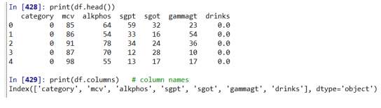
#train/test 셋 나눔
# Split the data into training/testing sets
train_X, test_X, train_y, test_y = \
train_test_split(df_X, df_y, test_size=0.3,\
random_state=1234)
#4. 모델 만듬
# Define learning model (basic)
model = DecisionTreeClassifier(random_state=1234)
#5. 모델 학습
# Train the model using the training sets
model.fit(train_X, train_y)
# performance evaluation
print('Train accuracy :',model.score(train_X, train_y))
print('Test accuracy :',model.score(test_X, test_y))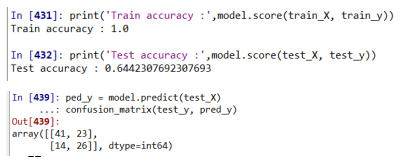
#6. 튜닝
# Define learning model (tuning)
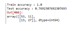
model = DecisionTreeClassifier(max_depth=4, random_state=1234)
# Train the model using the training sets
model.fit(train_X, train_y)
# performance evaluation
print('Train accuracy :',model.score(train_X, train_y))
print('Test accuracy :',model.score(test_X, test_y))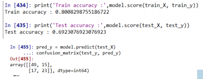
### 튜닝 후 test 정확도가 69%로 더 좋아진 것을 알 수 있다. 그러므로 매개변수를 잘 조절하면 모델의 성능이 좋아진다.
 visualize tree
export_graphviz(model, out_file='tree_model.dot', feature_names =
train_X.columns, class_names = 'category’, rounded = True,
proportion = False, precision = 2, filled = True)
(graph,) = pydot.graph_from_dot_file('tree_model.dot’,
encoding='UTF-8')
graph.write_png('decision_tree.png') # save tree image

#from IPython.display import Image
#Image(filename = 'decision_tree.png')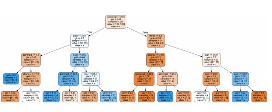
1.1.5 Hyper parameters
모델을 만들 때, 모델의 성능에 여향을 끼치는 매개변수들이다.
따라서 Hyper parameter를 어떻게 조절하냐가 중요하다. 그러나 매개변수가 20개 가까이 되므로 다 조절하기는 힘들다.
그러므로 몇개의 자료로 추린다.
- criterion : String, optional (default = "gini")
Decision Tree의 가지를 분리 할 때, 어떤 기준으로 정보 획득량을 계산하고 가지를 분리 할 것인지 정함
gini = entropy보다 빠르지만 한쪽으로 편향된 결과를 낼 수 있음
entropy = gini에 비해 조금 더 균형잡힌 모델을 만들 수 있다.
- max_depth : int or None, optional(default = None)
Decision Tree의 최대 깊이 제한을 줄 수 있음
사전 가지치기를 하고 voerfitting을 방지 할 수 있음
- min_sample_split : int, float optaional(default = 2)
노드에서 가지를 분리할 때 필요한 최소 sample 개수에 대한 제한을 줄 수 있음. 주어진 값에 type에 따라 다음과 같이 기능함
int -> 주어진 값 그대로 사용
float -> 0,1사이의 값을 줄 수 잇음,. cell(전체 데이터수 * min_sample_split)의 값을 사용함 - min_sample_leaf : int, float optaional(default = 2)
한 노드에서 가지고 있어야 할 최소 sample 개수에 대한 제한을 줄 수 있음.주어진 값에 type에 따라 다음과 같이 기능함
int -> 주어진 값 그대로 사용
float -> 0,1사이의 값을 줄 수 잇음,. cell전체 데이터수 * min_sample_leaf)의 값을 사용함 - max_features : int, float, string or None, optional(default = None)
Decision Tree model을 만들 때 사용할 수 있는 변수의 개수를 제한을 줄 수 있음
int -> 주어진 값 그대로 사용
flaot -> int(max_features * 총변수 개수) 사용
None -> 총 변수 개수 사용 - class_weight : dict, list of dict or "balanced", default=None
예측 할때 두개의 class의 중요도가 다른 경우가 있다.
예로 환자 판단시, 정상을 정상으로 진단하는 것보다 환자를 환자로 진단하는 것이 더 중요하다
그러므로 정상:환자 = 6:4 와 같이 비율을 정한다.
class_label: weight
1.2 Random Forest
- N개의 Decision Tree가 투표를 통해 결정하는 방식이다.
- Bagginf approach중 하나임. -> 여러 모델을 합쳐서 결론냄
- 주어진 데이터에서 랜덤하게 subset을 N번 sampling해서(좀 더 정확하게 observations와 features들을 랜덤하게 sampling) N개의 예측 모형을 생성
- 개별 예측 모형이 voting하는 방식으로 예측결과를 결정하여 Low Bias는 유지하고 High Variance는 줄임
- Random Forest는 이런 Bagging 계열의 가장 대표적이고 예측력 좋은 알고리즘
1.2.1 코드
from sklearn.ensemble import RandomForestClassifier
from sklearn.model_selection import train_test_split
from sklearn.metrics import confusion_matrix
import pandas as pd

# prepare the iris dataset
df = pd.read_csv('D:/data/liver.csv')
print(df.head())
print(df.columns) # column names
df_X = df.loc[:, df.columns != 'category']
df_y = df['category']

# Split the data into training/testing sets
train_X, test_X, train_y, test_y = \
train_test_split(df_X, df_y, test_size=0.3,\
random_state=1234)
# Define learning model (# of tree: 10) #################
model = RandomForestClassifier(n_estimators=10, random_state=1234) # n_estimators = 트리 수

# Train the model using the training sets
model.fit(train_X, train_y)

# performance evaluation
print('Train accuracy :', model.score(train_X, train_y))
print('Test accuracy :', model.score(test_X, test_y))
pred_y = model.predict(test_X)
confusion_matrix(test_y, pred_y)
# Define learning model (# of tree: 10) #################
model = RandomForestClassifier(n_estimators=10, random_state=1234)

# Train the model using the training sets
model.fit(train_X, train_y)

# performance evaluation
print('Train accuracy :', model.score(train_X, train_y))
print('Test accuracy :', model.score(test_X, test_y))
pred_y = model.predict(test_X)
confusion_matrix(test_y, pred_y)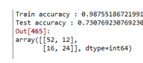
# Define learning model (# of tree: 50) #################
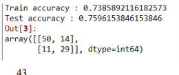
model = RandomForestClassifier(n_estimators=50, random_state=1234)
# Train the model using the training sets
model.fit(train_X, train_y)
# performance evaluation
print('Train accuracy :', model.score(train_X, train_y))
print('Test accuracy :', model.score(test_X, test_y))
pred_y = model.predict(test_X)
confusion_matrix(test_y, pred_y)tree 수를 50으로 늘리니까 정확도가 올라갔다.
Hyper parameters
- n_estimators : 생성하는 트리의 개수, 많을수록 성능이 좋아짐 이론적으론 500, 1000이면 충분
- max_feautures : 좋은 split을 하기위한 features의 개수
- Criterion : measure the quality of a split
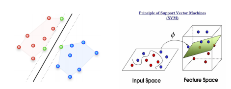
1.3 Support Vector Machine
이때까지는 tree 형태의 모델로 접근을 했다.
Support Vector Machine은 접근법이 다르다.
idea 1)
- finding maximum-margin hyperplane
모든 점 정보를 가지고 경계선을 찾는게 아니라 class 경계면에 있는 몇개의 점들로 경계선을 찾는다. - 데이터의 차원을 높이는 방법
차원을 높여서 찾는다.
- C - Support Vector Classification
학습시간이 sample 수(data set의 instance 수)의 제곱에 비례하여 많아짐
1.3.1 코드
from sklearn import svm
from sklearn.model_selection import train_test_split
from sklearn.metrics import confusion_matrix

import pandas as pd
import pydot

# prepare the iris dataset
df = pd.read_csv('D:/data/liver.csv')
df_X = df.loc[:, df.columns != 'category']
df_y = df['category']

# Split the data into training/testing sets
train_X, test_X, train_y, test_y = \
train_test_split(df_X, df_y, test_size=0.3,\
random_state=1234)
# Define learning model (basic)
#####################################
model = svm.SVC()
# Train the model using the training sets
model.fit(train_X, train_y)
# performance evaluation
print('Train accuracy :', model.score(train_X, train_y))
print('Test accuracy :', model.score(test_X, test_y))
pred_y = model.predict(test_X)
confusion_matrix(test_y, pred_y)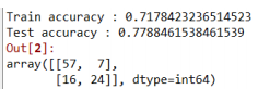
# Define learning model (poly kernel) ############
model = svm.SVC(kernel='poly')

# Train the model using the training sets
model.fit(train_X, train_y)

# performance evaluation
print('Train accuracy :', model.score(train_X, train_y))
print('Test accuracy :', model.score(test_X, test_y))
pred_y = model.predict(test_X)
confusion_matrix(test_y, pred_y)
정확도가 낮아졌다.
1.3.3 Hyper parameter
- c: float, deault =1.0
Regularization parameter
과적합을 조절(일어나지 않게) - kernel : linear, poly, rbf, sigmoid, precomputerd default = 'rbf'
차원 변경 - degree : int, default = 3
커널에 따라 달라짐 - gamma : scale, auto or float default = 'scale'
'rbf', 'poly', 'sigmoid' 지원
1.3.4 SVM 장단점
장점
- 범주나 수치데이터 보두에 사용가능
- 노이즈 데이터에 영향을 크게 받지 않고 overfitting이 잘 일어나지 않음
- 경계면의 몇개의 점만 사용하므로
- 높은 정확도
단점
- 최적의 모델을 찾기 위해 커널과 기타 hyper parameter의 여러 조합ㅇ르 테스트해보아야한다.
- 입력 데이터셋이 feature 수와 데이터 sample 수가 많으면 훈련시간이 많이 소요될 수 있다.
- 모델의 해석이 불가능하진 않지만 어렵다.
1.4 xgboost
예측력이 가장 좋지만 복잡하다.
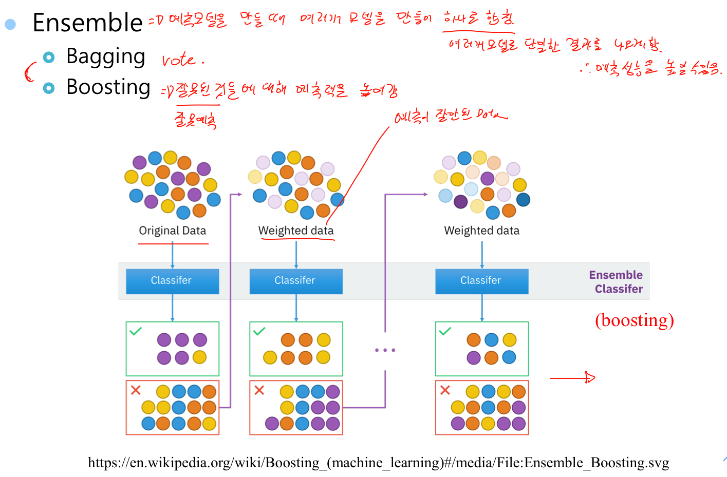
- Ensemble => 예측 모델을 만들때 여러개 모데ㅐㄹ을 만들어 하나로 합친다. 여러개 모델로 단일한 결과를 나오게 한다. 예측 성능을 높일 수 있다.
- Bagging => 투표로 결과 도출
- Boosting =>잘못 예측된 것들에 대해 예측력을 높여줌
728x90
반응형
'공부 > 딥러닝' 카테고리의 다른 글
| CIFAR-10 의 레이블중 하나를 예측 (0) | 2021.05.09 |
|---|---|
| classification 경진대회 (0) | 2021.05.03 |
| 딥러닝 4 (0) | 2020.10.29 |
| 딥러닝 2 (0) | 2020.09.29 |
| 딥러닝 1 (0) | 2020.09.25 |

아상관없어