


- trainset.csv 파일을 이용하여 classification 모델 생성
- 모델을 이용하여 testset.csv 파일의 자료에 대한 class 예측
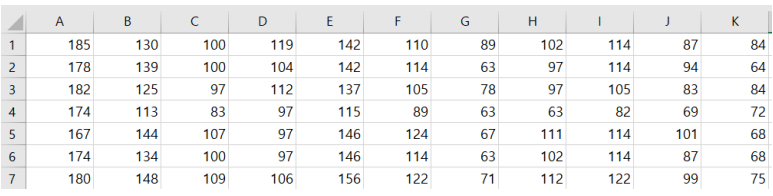
trainset.csv

(A열이 class label이다.)
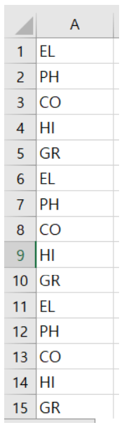
testset.csv
- 예측결과 포맷
=========================================================================
model development process는 [Feature Selection -> Algorithm Selection -> Hyper parameter tuning] 순이므로, 먼저 어떠한 Feature을 고를 것인지 결정하였습니다.
Feature Selection 방법으로 강의에서 배운 filter method, backward elimination, forward selection 세가지 방법으로 테스트를 하였습니다. Feature selection을 하기 위해 model을 선택하여야 했는데, 이는 강의에서 배운 model comparison을 통하여 선정하였습니다.
기존에 배운 분류 알고리즘인 DecisionTreeClassifier, KNeighborsClassifier, RandomForestClassifier, SVC 외에 검색을 통하여 몇 가지 알고리즘을 추가하였습니다. 자주 사용되는 Xgboost, xgboost의 느린 단점을 보완한 LightGBM을 추가하여 비교를 하였습니다. (pip install 명령어를 사용하여 설치함)
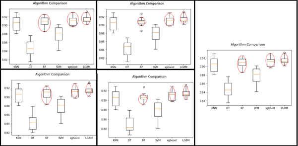
5번 반복하여 비교한 결과 RandomForest와 xgboost, LightGBM이 모델 변동폭이 작고 정확도도 높은 것을 알 수 있어 이 3가지 모델을 사용하여 비교해보기로 하였습니다.
from sklearn.model_selection import RandomizedSearchCV
from sklearn.model_selection import cross_val_score
from sklearn.model_selection import train_test_split
from xgboost import plot_importance

# Model comparison
import matplotlib.pyplot as plt
from sklearn import model_selection

# from sklearn.linear_model import LogisticRegression
from sklearn.tree import DecisionTreeClassifier
from sklearn.neighbors import KNeighborsClassifier
from sklearn.ensemble import RandomForestClassifier
from sklearn.svm import SVC
from xgboost import XGBClassifier
from lightgbm import LGBMClassifier
from sklearn.preprocessing import LabelEncoder
from sklearn.model_selection import KFold
from sklearn.metrics import accuracy_score
import pandas as pd
import numpy as np
import pprint as pp

#1. 데이터 셋 준비
data = pd.read_csv('C:\dataset/trainset.csv')

#2. 설명변수 반응 변수 나눔
data_x = data.iloc[:, 1:32]
data_y = data.iloc[:, 0]

# train, test 나눔
train_X, test_X, train_y, test_y = train_test_split(data_x, data_y, test_size=0.3,random_state=1234)


# prepare configuration for cross validation test harness
seed = 7

# prepare models
models = []
models.append(('KNN', KNeighborsClassifier()))
models.append(('DT', DecisionTreeClassifier()))
models.append(('RF', RandomForestClassifier()))
models.append(('SVM', SVC()))
models.append(('xgboost', XGBClassifier()))
models.append(('LGBM', LGBMClassifier()))
results = []
names = []
scoring = 'accuracy'

for name, model in models:
    kfold = model_selection.KFold(n_splits=10, random_state=seed, shuffle=True)
    cv_results = model_selection.cross_val_score(model, data_x, data_y, cv=kfold, scoring=scoring)
    results.append(cv_results)
    names.append(name)
    msg = "%s: %f (%f)" % (name, cv_results.mean(), cv_results.std())
    print(msg)

print(results)

# average accuracy of classifiers
for i in range(0,len(results)):
    print(names[i] + "\t" + str(round(np.mean(results[i]),4)))

# boxplot algorithm comparison
fig = plt.figure()
fig.suptitle('Algorithm Comparison')
ax = fig.add_subplot(111)
plt.boxplot(results)
ax.set_xticklabels(names)
plt.show()
그리고 filter method, backward elimination, forward selection을 통하여 feature을 선정하였습니다.
(먼저 데이터 셋의 column name이 없어 0부터 숫자를 순서대로 할당하여 보기 편하게 하였습니다. Backward n_features_to_select=4, Cv=5)
[모델 선택하기 위해 비교]
LighGBM의 경우
[filter method]
“0.9159”
[backward elimination]
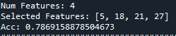
“0.7869”
[forward selection]
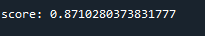
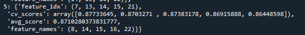
“0.871”
RandomForest의 경우
[filter method]

“0.909”
[backward elimination]
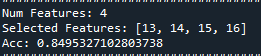
“0.849”
[Forward selection]
“0.871”
Xgboost의 경우
[filter method]

“0.907”
[backward elimination]

“0.850”
[Forward selection]
“0.872”
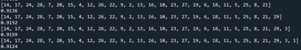
각기 다른 모델을 사용해도 feature의 중요도는 바뀌질 않으니 빠른 lightGBM 모델로 backward, forward selection에서 각 인자 n_features_to_select, k_features의 수를 filter method 에서 얻은 데이터를 바탕으로 수정하여 한번 더 테스트 하였습니다.
Filter method의 결과를 보면 선택하는 feature의 수가 많아질수록 정확도가 높아지므로 개수를 크게 변화가 없어지는 21개부터 30개까지 테스트를 해보았습니다.
하지만 forward selction을 할 경우 시간이 오래 걸리고 컴퓨터도 간헐적으로 멈추어 backward elimination으로 테스트하였습니다.
# Feature selection Example
import pandas as pd
import numpy as np
from sklearn.linear_model import LogisticRegression
from sklearn.model_selection import cross_val_score
from sklearn.tree import DecisionTreeClassifier
from sklearn.neighbors import KNeighborsClassifier
from sklearn.ensemble import RandomForestClassifier
from sklearn.svm import SVC
from sklearn.preprocessing import LabelEncoder
#from xgboost import XGBClassifier
from lightgbm import LGBMClassifier
#1. 데이터 셋 준비
name = []
for i in range(0,32):
name.append(i)
data = pd.read_csv('C:\dataset/trainset.csv', names = name)
print(data.head())
#2. 설명변수 반응 변수 나눔
data_x = data.iloc[:, 1:32]
data_y = data.iloc[:, 0]
# whole features
model = LGBMClassifier()
scores = cross_val_score(model, data_x, data_y, cv=5)
print("Acc: "+str(scores.mean()))
print('######################################################################')
print('# feature selection by filter method')
print('######################################################################')
######################################################################
# feature selection by filter method
######################################################################
# feature evaluation method : chi-square
from sklearn.feature_selection import SelectKBest
from sklearn.feature_selection import chi2
test = SelectKBest(score_func=chi2, k=data_x.shape[1])
fit = test.fit(data_x, data_y)
# summarize evaluation scores
print(np.round(fit.scores_, 3)) #소수점 3자리까지 반올림
f_order = np.argsort(-fit.scores_) # sort index by decreasing order
sorted_columns = data.columns[f_order]
f_order
data_x.shape[1]
# test classification accuracy by selected features
model = XGBClassifier()
for i in range(0, data_x.shape[1]):
fs = sorted_columns[0:i]
data_x_selected = data_x[fs]
scores = cross_val_score(model, data_x_selected, data_y, cv=5)
print(fs.tolist())
print(np.round(scores.mean(), 4))
'''
for i in range(20, 31):
print('index = ', i)
'''
######################################################################
# Backward elimination (Recursive Feature Elimination)
######################################################################
from sklearn.feature_selection import RFE
model = LGBMClassifier()
rfe = RFE(model, n_features_to_select=i)
fit = rfe.fit(data_x, data_y)
print("Num Features: %d" % fit.n_features_)
fs = data_x.columns[fit.support_].tolist() # selected features
print("Selected Features: %s" % fs)
scores = cross_val_score(model, data_x[fs], data_y, cv=5)
print("Acc: "+str(scores.mean()))
print('######################################################################')
print('# Forward selection')
print('######################################################################')
######################################################################
# Forward selection
######################################################################
# please install 'mlxtend' moudle
from mlxtend.feature_selection import SequentialFeatureSelector as SFS
model = LGBMClassifier()
sfs1 = SFS(model, k_features=i, n_jobs=-1, scoring='accuracy', cv=5)
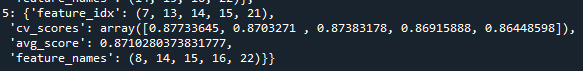
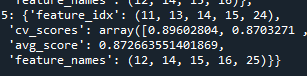
sfs1 = sfs1.fit(data_x, data_y, custom_feature_names=data_x.columns)
sfs1.subsets_ # selection process
sfs1.k_feature_idx_ # selected feature index
print(sfs1.k_feature_names_)# selected feature name
Backward elimination을 하였을 때
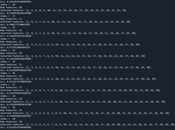
Feature을 25개 사용하면 정확도가 0.9165으로 가장 좋았지만, 나머지와 비교하였을 때 filter method도 그러하듯이 feature 개수에 따른 큰 차이를 보여주지 못하여 테스트 시 모든 feature들을 사용하기로 결정하였습니다.
이제 hyperparameter 튜닝을 하기 전 각 모델별로 테스트를 해보았다.
Feature을 선정하기 위한 과정에서 model도 함께 선정하였으므로 다음으로 hyperparameter tuning을 진행하였습니다. Hyper parameter를 찾기 위해 RandomizedSearchCV 방법을 사용하였습니다.
(다른 최적화 방법 BaysianOptimizaion을 찾았으나 정확한 사용법을 익히지 못하여 RandomizedSearchCV 방법을 사용하였습니다.
또한 autosklearn을 통하여 최적의 모델을 찾고 hyper parameter 최적값을 찾는 과정을 자동으로 해주려 하였으나, 다음의 글을 찾아“Anaconda does not ship auto-sklearn, and there are no conda packages for auto-sklearn” 이 방법은 해보지 못하였습니다.
-Xgboost
max_depth(int, default: 3): 기본 학습자를 위한 최대 트리 깊이
learning_rate(float, default: 0.1) : Boosting 학습률
n_estimators(int, default: 100) : fit하기 위한 Boosted tree의 수
silent(boolean, default: True : Boosting을 실행하는 동안 메시지를 print할지 여부
objective(string or callable, default:’reg:linear’) : 학습할 Objective Function 사용
booster(string, default: ‘gbtree’): Booster가 사용할 모드 gbtree, gblinear, dart
nthread(int, default: ‘None’): xgboost를 실행하는데 사용할 병렬 스레드 수
- xgboost.XGBClassifier(nthread=20)
n_jobs(int, default: 1): xgboost를 실행하는데 사용할 병렬 스레드 수
gamma(float, default: 0): 트리의 leaf 노드에 추가 파티션(partition)을 만들때 최소 손실 감소(Minimum loss reduction)가 필요하다.
min_child_weight(int, default: 1): Child 노드에 필요한 instance weight(hessian) 최소 합계
max_delta_step(int): 각 Tree의 가중치(Weight) 추정을 허용하는 최대 Delta 단계
subsample(float): 학습(Training) Instance의 Subsample 비율
colsample_bytree(float): 각 Tree를 구성할 때 column의 Subsample 비율
colsample_bylevel(float): 각 Tree의 Level에서 분할(split)에 대한 column의 Subsample
처음햇을 때
max_depth를 늘리니 향상되는 것을 알 수 있었다.
따라서 max_depth를 더 늘려 테스트해보려 하였지만, 실수로 n_estiators를 np.linspace(start = 200, stop = 10000, num = 21)와 같이 늘려서 테스트 하였다.
시간은 2시간 가량 걸렸지만, n_estimators의 값은 크게 영향이 없다는 것을 알았다.
Max_depth값이 늘어났을 때 성능이 향상되는 것을 알 수 있었다.
np.linspace(4000, 10000, num = 11)로 바꾸어 하였을 때,
비슷한 향상 폭을 보여주었다.
-RandomForest
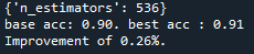
예제코드와 같이 실행을 하면
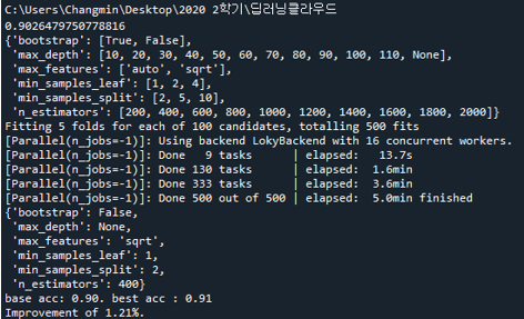
1.21%의 향상을 얻을 수 있었습니다.
위와 같이 각 모델에 대해 HyperParameter를 진행하려하였으나,
tuning할 parameter들의 수가 많고 tuning을 하는 과정도 상당한 시간이 걸려,
시간 비용을 줄이고자 분산이 적고 예측력이 세가지 모델 중 가장 좋은 LightGBM을 선택하여 hyper parameter tuning을 하고 테스트를 진행하였습니다.
=========================================================================
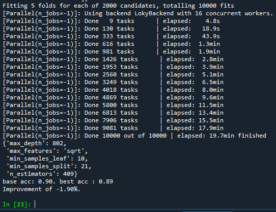
초반에는 여러 데이터들의 범위를 바꾸어 가면서 테스트를 하였습니다.
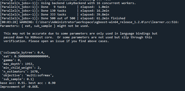
2000 candidates를 하였지만 시간대비 좋지 않은 결과를 얻었다.
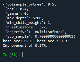
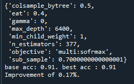
Xboost에서 max_depth가 커지면서 좋아진 것을 보고 LightGBM에서도 값을 크게 잡아서 테스트를 하였다.
Candidates는 100이지만 성능이 더 좋아진 것으로 보아 candidate를 크게 잡을 필요가 없다고 생각하였습니다.
그리고 num_leaves를 바꾸어 테스트하였으나 결과에 변화가 없는 것으로 보아 num_leaves는 큰 영향을 끼치지 않는 것으로 확인했다.
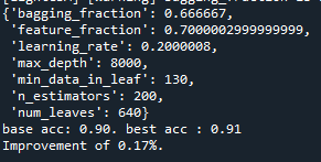
min_data_in_leaf가 커지면 향상 폭이 줄어드는 것을 확인하였다.
따라서 max_depth가 크면 향상 폭이 가장 좋아지는 것으로 판단하였다.
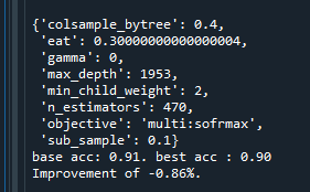
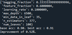
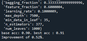
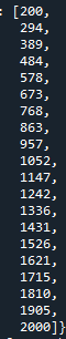
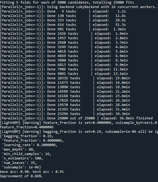
parameter들을 범위를 넓혀 가면서 테스트를 하였다.
범위를 넓게 한 경우
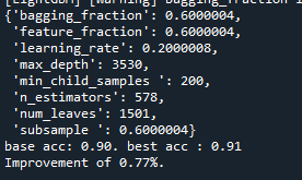
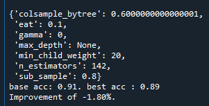
그리고 default parameter를 사용할 때와 0.82%의 향상이 있었던 파라미터를 사용하여 테스트해보았습니다.
Default의 경우 0.93이 나왔고, 향상된 파라미터를 사용할 경우 0.90으로 줄어들었습니다. 과적합이 의심되어 max_depth값을 낮추어 다시 테스트하니 0.93이 나온 것을 알 수 있었습니다. 따라서 과적합과 같은 경우를 고려하기 위하여 과적합을 줄일 수 있는 요소를 찾아보았습니다.
https://greeksharifa.github.io/machine_learning/2019/12/09/Light-GBM/와http://machinelearningkorea.com/2019/09/29/lightgbm-%ED%8C%8C%EB%9D%BC%EB%AF%B8%ED%84%B0/를 참고하여 사용할 파라미터를 선정하였습니다.
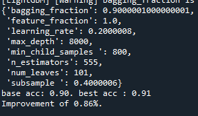
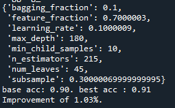
그리고 여러 parameter들을 종합적으로 테스트를 하면 각 요소들이 얼만큼 차이를 내는지 파악하기 힘들어 parameter 하나씩 테스트를 하였습니다.

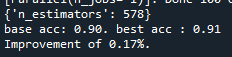
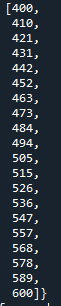
다음과 같이 범위를 좁혀나가며 best Parameter에 근접한 범위로 좁혀가면서 최적 값을 찾아보았습니다. 그리고 과적합을 조절할 파라미터들은 max_depth와 함께 테스트하였습니다.
하지만 다른 파라미터들과 함께 테스트하였을 때 좋지 않은 결과를 보여주기도 하였습니다.
사이트를 통하여 테스트시 0.93

적절한 max_depth를 찾으려 하였으나, 초기에 max_depth값 테스트를 해보기위해 설정했던 max_depth = 90, learning_rate = 0.1, n_estimators = 300이 가장 좋은 결과를 보여주었습니다. 아마 과적합이 일어나면서 확률이 좋아진 것으로 예상합니다. 과적합을 줄이면서 좋은 성능을 내는 파라미터를 찾기 어려웠습니다. 따라서 n_iter의 값을 늘리고 max_depth, n_estimators의 값을 줄여서 테스트 하였습니다.
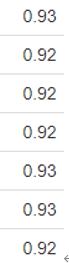
여러 번 testset으로 예측한 결과 max_depth와 learning_rate, n_estimators의 값을 변경한 경우가 0.93으로 더 좋은 예측을 보여주어 다른 값보다 이 3가지 값을 변경시켜 더 테스트 해보기로 하였습니다. 범위를 넓히고 과적합을 줄이기 위해 범위를 줄이면서, n_iter은 1000으로 늘려 여러 값들을 테스트해보았습니다.
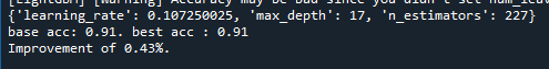


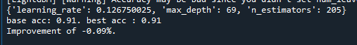

그래도 변화가 없어 0.43%가 나왔던 범위를 선택하고 나머지 parameter들을 추가하여 다시 테스트해 보았습니다.
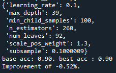

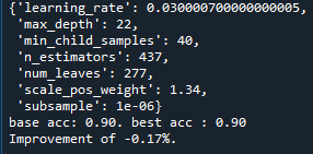

0.92로 향상은 없었습니다.
Hyper parameter값들을 여러가지로 조정해보고 testset을 적용하여 정확도를 보았을때, acc : 0.929039301310044 가 가장 좋은 결과를 보여주었습니다.
###HYPERPAMETER TUNING####
from sklearn.model_selection import RandomizedSearchCV
from sklearn.model_selection import cross_val_score
from sklearn.model_selection import train_test_split
# Model comparison
import matplotlib.pyplot as plt
from sklearn import model_selection
# from sklearn.linear_model import LogisticRegression
from sklearn.tree import DecisionTreeClassifier
from sklearn.neighbors import KNeighborsClassifier
from sklearn.ensemble import RandomForestClassifier
from sklearn.svm import SVC
from sklearn.preprocessing import LabelEncoder
from xgboost import XGBClassifier
import lightgbm as lgb
from lightgbm import LGBMClassifier
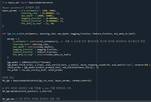
from bayes_opt import BayesianOptimization
from hyperopt import fmin, tpe, hp
import pandas as pd
import numpy as np
import pprint as pp
'''
HI, PH, GR, PH, EL, MI, PH, MI, CO, EL, GR....
1. feature selecion
2. algorithm selection
3. hyper parameter tuning
randomizedserchcv 가 조합을 자동으로 골라주고, 시간이 줄어드므로 사용함.
'''
#1. 데이터 셋 준비
data = pd.read_csv('C:\dataset/trainset.csv')
#2. 설명변수 반응 변수 나눔
data_x = data.iloc[:, 1:32]
data_y = data.iloc[:, 0]
data_x
# train, test 나눔
train_X, test_X, train_y, test_y = train_test_split(data_x, data_y, test_size=0.3, random_state=1234)
base_model = LGBMClassifier(random_state=1234)
base_model.fit(train_X, train_y)
base_accuracy = base_model.score(test_X, test_y)
print(base_accuracy)
n_estimators = [int(x) for x in np.linspace(start = 200, stop = 600, num = 41)]
# Maximum number of levels in tree
max_depth = [int(x) for x in np.linspace(1, 400, num = 41)]
#하나의 트리가 가지는 최대 리프 개수
#num_leaves = [int(x) for x in np.linspace(2, 1000, num = 31)]
#리프 노드가 되기 위한 최소한의 샘플 데이터 수
#min_child_samples = [int(x) for x in np.linspace(1, 100, num = 11)]
learning_rate = [float(x) for x in np.linspace(0.000001, 0.5, num = 41)]
#데이터 샘플링 비율 0이되면 안됨
#bagging_fraction = [float(x) for x in np.linspace(0.1, 1, num = 11)]
#개별 트리 학습시 선택되는 피처 비율 - 과적합 방지
#feature_fraction = [float(x) for x in np.linspace(0.000001, 1, num = 11)]
#과적합을 제어하기 위해 데이터를 샘플링하는 비율
#subsample = [float(x) for x in np.linspace(0.000001, 1, num = 11)
#metric = ['multiclass']
# Create the random grid
random_grid = {'n_estimators' : n_estimators,
'max_depth' : max_depth,
#'feature_fraction': feature_fraction,
#'subsample' : subsample,
'learning_rate' : learning_rate
#'bagging_fraction' : bagging_fraction,
#'num_leaves' : num_leaves,
#'min_child_samples' : min_child_samples,
# 'metric' : metric
}
pp.pprint(random_grid)
'learning_rate' : learning_rate
#'bagging_fraction' : bagging_fraction,
#'num_leaves' : num_leaves,
#'min_child_samples' : min_child_samples,
# 'metric' : metric
}
pp.pprint(random_grid)
# Use the random grid to search for best hyperparameters
rf = LGBMClassifier(random_state=1234)
rf_random = RandomizedSearchCV(estimator = rf, param_distributions = random_grid, n_iter = 1000, cv = 5, verbose=2, random_state=42, n_jobs = -1)
# Fit the random search model
rf_random.fit(train_X, train_y)
# best parameters
# best_params에 최적 조합이 저장됨
pp.pprint(rf_random.best_params_)
# best model
#best_estimator => 최적 조합을 적용해서 만들어진 모델
best_random_model = rf_random.best_estimator_
best_random_accuracy = best_random_model.score(test_X, test_y)
print('base acc: {0:0.2f}. best acc : {1:0.2f}'.format( \
base_accuracy, best_random_accuracy))
print('Improvement of {:0.2f}%.'.format( 100 * \
(best_random_accuracy - base_accuracy) / base_accuracy))
######testset save to csv#######
from lightgbm import LGBMClassifier
import pandas as pd
import numpy as np

#1. 데이터 셋 준비
data = pd.read_csv('C:\dataset/trainset.csv', header=None)
test_x = pd.read_csv('C:\dataset/testset.csv', header=None)

data.shape
test_x.shape
#2. 설명변수 반응 변수 나눔
data_x = data.iloc[:, 1:32]
data_y = data.iloc[:, 0]

data_x
data_y

model = LGBMClassifier(learning_rate = 0.1, max_depth = 90, n_estimators = 300)
model.fit(data_x, data_y)

pred_y = model.predict(test_x)

result = pd.DataFrame(pred_y)
result.to_csv('lightgbm.csv', header=None, index=False)
후기)
먼저 그래프로 모델을 비교하여 해당 데이터에 어떤 모델이 가장 잘 맞는지 고르는 것이 전반적인 예측율에 많은 영향을 끼친다고 느꼈다. 그리고 적절한 feature을 찾기 위해 시간이 빠른 모델을 사용하여 테스트를 하면 시간을 줄일 수 있고 hyper parameter를 찾기 위한 여러가지 방법들을 알게 되었다.
이번 경진대회에서는 RandomizedSearchCV를 사용하였다. 이 방법으로 적절한 hyper parameter를 찾기 위해 parameter 별로 값을 바꾸어 테스트를 해보고, 여러 parameter들을 동시에 바꾸어 가며 테스트를 하였다.
또한 n_iter을 높일수록 과적합을 줄여 향상이 더 줄어들 수 있다는 것도 알게 되었다. 하지만 적절한 값을 찾는 것이 매우 힘들었다. Parameter를 바꿀 때 이것이 향상되었는지 과적합인지, 과소적합인지를 구분하기가 힘들었다.
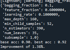
처음에 1.38%의 향상을 보았지만 그 값은 과적합으로 인해 예측은 좋지 못하였고, 오히려 max_depth를 낮추니 결과가 좋아지는 경우를 보았다. 또한 test_size 비율을 바꿔가며 나온 결과값을 테스트해보았지만 좋은 결과를 얻기는 어려웠다.
따라서 이런 튜닝을 하는 과정은 소모적이며 때론 2시간 이상이 걸릴 만큼, 시간이 많이 들고 적절한 값을 찾는 것은 감에 의존하고 우연에 의존한다는 생각을 하였다. 이런 과정을 편하게 해주는 방법들이 없을까 찾아보았고, hyper parameter가 변경될 때마다 정확도의 변화를 그래프로 보여주던가, 과적합을 판단할 수 있게 과적합 수치도 함께 보여준다면 더 편리할 것이라 생각하였다.
AutoML은 데이터의 특성에 따라 좋은 알고리즘과 어울리는 파라미터들을 자동화하여 찾아준다.
그 중 Auto-sklearn라는 방법이 있다. 데이터가 들어오면, 데이터에 맞을만한 알고리즘, parameter를 알려주는 meta-learning process를 진행하고 이 결과로 알고리즘과 parameter set들을 추천해 준다. 그 후 앙상블 기법을 활용해 추천된 알고리즘, parameter set들의 최적화를 진행합니다. 하지만 “Anaconda does not ship auto-sklearn, and there are no conda packages for auto-sklearn” 와 같은 답변을 얻어 실제로 해보진 못하였다.
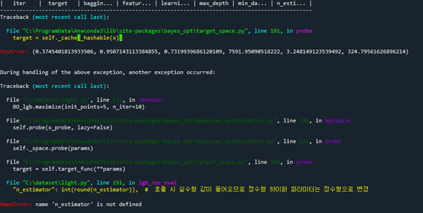
그리고 Bayesian Optimization을 통하여 hyper parameter의 최적값을 탐색할 수 있다. Bayesian Optimization은 매 회 새로운 hyper parameter값에 대한 조사를 수행할 시, 사전지식을 충분히 반영하면서 전체적인 탐색 과정을 체계적으로 수행할 수 있는 방법론이다. 따라서 이 방법을 통하여 hyper parameter를 찾으려 하였다. 하지만 완벽히 이해하지 못하였고, 관련 자료를 많이 찾지 못하여 사용법과 에러에 대한 원인을 찾지 못하였다.
'공부 > 딥러닝' 카테고리의 다른 글
| 흉부 X-ray 사진으로 폐렴 진단 모델 (0) | 2021.05.09 |
|---|---|
| CIFAR-10 의 레이블중 하나를 예측 (0) | 2021.05.09 |
| 딥러닝 4 (0) | 2020.10.29 |
| 딥러닝 3 (0) | 2020.10.09 |
| 딥러닝 2 (0) | 2020.09.29 |

아상관없어